4.1.1 사이킷런을 통해 학습과 예측에 사용할 데이터셋 나누기
- 사이킷런에서 지원되는 train_test_split를 통해 학습과 예측에 사용될 데이터 셋을 나눌 수 있다.
from sklearn.model_selection import train_test_split
train_test_split(arrays, test_size, train_size, random_state, shuffle, stratify)
파라미터 설명
arrays: 분할시킬 데이터를 입력(리스트,배열,데이터 프레임)
test_size: 테스트 데이터셋의 비율(default = 0.25)
train_size: 학습 데이터셋의 비율( default = test_size의 나머지)
random_state: 데이터 분할시 셔플이 이루어지는데 이를 위한 시드값(강의에서는 42로 고정함)
shuffle: 셔플을 할지 말지 여부를 결정
stratify: 지정한 Data의 비율을 유지한다. 예를 들어, Label Set인 Y가 25%의 0과 75%의 1로 이루어진 Binary Set일 때, stratify=Y로 설정하면 나누어진 데이터셋들도 0과 1을 각각 25%, 75%로 유지한 채 분할된다.
from sklearn.model_selection import train_test_split
X_train, X_test, y_train, y_test = train_test_split(
X, y, test_size=0.2, random_state=42)
실제 코드
4.1.2 ~ 4.1.3 max_depth값을 바꿔가며 decision tree로 학습 ,예측
from sklearn.metrics import accuracy_score

for max_depth in range(3, 12):
    model = DecisionTreeClassifier(max_depth=max_depth, random_state=42)
    y_predict = model.fit(X_train, y_train).predict(X_test)
    score = accuracy_score(y_test, y_predict) * 100
    print(max_depth, score)
실제 코드
해당 코드는 max_depth의 깊이를 바꿔가며 모델의 정확도를 비교하는 코드이다, 주의해야할 점은 max_depth의 깊이가 길어질수록 과대적합이 일어날 수 있고, 깊이가 너무 얕으면 언더피팅이 일어날 수 있다.
지니 계수(Gini index) : 불순도를 측정하는 척도로서 데이터의 통계적 분산정도를 정량화해서 표현한 값이다.

지니 계수의 식
S: 이미 발생한 사건들 c: 사건의 개수 p: 전체 사건 중에서 특정 사건의 수 --> 지니 계수가 높을 수록 데이터가 분산되어 있음을 의미
** 또 다른 분할 계수
엔트로피 계수: 정보 이론에서, 정보의 불확실함의 정도를 나타내는 양

엔트로피 계수의 식

max_depth를 바꿔가며 도출한 정확도
4.1.4 GridSearchCV를 사용해서 최적의 하이퍼 파리미터 값 찾기
그리드 서치는 가능한 모든 하이퍼파라미터 조합에 대해 모델을 평가하고, 가장 성능이 우수한 조합을 선택합니다. 이를 위해 미리 정의된 하이퍼파라미터 값들의 조합을 그리드(grid) 형태로 만들어 이를 차례대로 모델에 적용하고 성능을 측정합니다. 그러면서 최적의 하이퍼파라미터 조합을 찾게 됩니다.
보통 그리드 서치는 교차 검증(cross-validation)과 함께 사용됩니다. 교차 검증은 데이터를 여러 개의 fold로 나누어 모델을 여러 번 학습하고 평가하여 모델의 일반화 성능을 더 정확하게 측정하는 기법입니다. 그리드 서치는 이러한 교차 검증을 통해 각 하이퍼파라미터 조합의 성능을 평가하고 가장 좋은 조합을 선택합니다.
Grid Search
Grid Search는 머신 러닝 모델에서 최적의 하이퍼파라미터(hyperparameter) 조합을 찾기 위한 기술 중 하나이다. 하이퍼파라미터란 모델 학습 전에 설정해야 하는 매개변수로, max_depth, max_features 등이 있다. Grid Search의 옵션으로는 estimator, param_grid, scoring,n_jobs 등이 있다.
또 cv라는 옵션이 있다. 기본적으로 5 폴더를 사용하여 cross validation을 한다.

여기서 cross validation은 train 데이터셋을 여러 fold로 나누어 평균을 내는 방법이다.
처음에 나눈 8:2 (train: test) 중 그 train데이터셋을 여러개로 나누는 것이다. 그리고 각 폴드를 test data를 통해 score을 내고 그것들의 점수의 평균을 내면 더 결과가 근사해질것이다.
gird search는 다음과 같이 불러오면 된다.
from sklearn.model_selection import GirdSearchCV

GridSearchCV()
옵션을 지정해주어야 오류가 나지 않는다.
estimator, param_grid, n_jobs, cv, verbose에 대한 옵션을 설정해보겠다.
estimator은 model 이다.
model = DecisionTreeClassifier(random_state=42)
param_grid에는 튜닝하고 싶은 파라미터 정보를 넣는다.
param_grid = {"max_depth":range(3,12), "max_features'" : [0.3,0.5,0.7,0.9,1.0]}
max_features는 일부 feature만 사용하고 싶을 때 사용한다. 1은 전체라는 뜻이다.
n_jobs는 -1로 설정하여 사용 가능한 모든 장비를 학습에 이용한다.
cv는 cross validation을 5개로 나눈다.
verbose를 1로 하여 로그를 찍으면서 학습을 합니다. 0이면 로그를 출력하지 않는다.
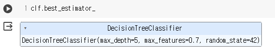
clf. 을 하면 best_estimator_, best_score, cv_results_등을 알 수 있다.
clf.best_params_를 보면 가장 성능이 좋은 파라미터를 찾아준다.
max_depth와 max_features에 대한 정보를 볼 수 있다.

clf.best_estimator은 가장 좋은 성능을 내는 파라미터 조합 전체를 알려준다.
clf.best_score_하면 가장 좋은 점수를 알려준다.

cv_results_는 cross validation결과를 반환해준다. 이때 보기 불편하니 데이터프레임 형식으로 바꾸어주면 편하다.
pd.DataFrame(clf.cv_results_).sort_values(by="rank_test_score").head()
score을 내림차순으로 보도록 옵션을 추가하였다.

데이터프레임을 확인하면 split이 5개로 나누어져있는 것을 확인할 수 있다. 그리고 그 split의 score를 평균 낸 값도 확인할 수 있다.
이러한 grid search로 예측한 값을 확인해보자.
이러한 score은 폴드 1~5까지 평균 낸 값을 통해 가장 좋은 파라미터 값을 찾았다. 그리고 그것을 적용하니 더 좋은 스코어가 나온 것을 확인할 수 있다.
4.1.5 RandomSearchCV를 사용해서 최적의 하이퍼 파라미터값 찾기
Grid Search는 우리가 설정한 범위 안에서만 parameter을 탐색하지만 Random Search는 좋은 성능을 낼 수 있는 랜덤값을 탐색한다.
RandomSearchCV를 불러와보자.
from sklearn.model_selection import RandomizedSearchCV

clf = RandomizedSearchCV()
다음과 같은 코드를 통해 RandomSearchCV를 불러왔다.
이제 emstimator, param_distributions, n_iter, scoring, n_jobs와 같은 옵션을 설정해 보자.
from sklearn.model_selection import RandomizedSearchCV

clf = RandomizedSearchCV(model,param_distributions, n_iter=1000, scoring="accuracy", n_jobs=-1, cv=5,
                   random_state=42)

clf.fit(X_train, y_train)
model은 위에서 한 설정과 같다.
param_distribution에서는 min_samples_split, max_depth와 max_features를 지정해보겠다.
max_depth = np.random.randint(3, 20, 10)
max_depth
max_features = np.random.uniform(0.7, 1.0, 100)
param_distributions = {"max_depth" :max_depth,
"max_features": max_features,
"min_samples_split" : list(range(2, 7))
}
param_distributions파라미터를 찾을 때 범위를 랜덤으로 지정하면 grid search와 다르게 구할 수 있다.
np.random.randint(3,20,10)이면 3부터 20까지 랜덤한 숫자 10개를 뽑아낸다.
min_samples_split은 노드를 분할하기 위해 필요한 최소 샘플 수를 설정하는 것이다.
n_iter은 =1000 일 경우 1000번을 돌면서 가장 좋은 하이퍼파라미터를 찾겠다는 것이다.
scoring은 accuracy를 사용하고, n_jobs=-1로 설정하여 모든 자원을 사용하도록 설정한다.
cv는 위에서 설명한 것과 동일하다.
위의 코드를 실행시키고 best params와 best score을 알아보자
clf.best_params_max depth는 9, max features는 0.7이 나온다.
clf.best_score_0.85177이 나온다.
pd.DataFrame(clf.cv_Results_).sort_values(by="rank_test_score")위 코드를 통해 실행시킨 결과를 확인하고, 좋은 파라미터의 결과를 확인 후 위에 설정한 범위들을 수정할 수 있다.
이렇게 좋은 스코어를 찾기 위해 범위를 조정해보는 것이 중요하다.
Grid Search보다 더 많은 값을 랜덤하게 학습시킬 수 있는 것이 Random Search이다.
4.2.1 랜덤포레스트 사용하기
DecisionTree 알고리즘 뿐만 아니라 랜덤 포레스트로 다양한 알고리즘을 사용하고, 이를 통해 모델의 성능을 올려보자.
먼저 DecisionTree로 모델을 만들어보자.
from sklearn.tree import DecisionTreeClassifier

model = DecisionTreeClassifier(random_state=42)
model
(학습을 진행하는 내용은 같기에 생략한다.)
해당 DecisionTree만 사용할 때의 다르게 예측한 갯수와 정확도는
(y_predict!=y_test).sum()28
from sklearn.metrics import accuracy_score

accuracy_score(y_test, y_predict)
0.8181818181818182
다음과 같은 값이 나온다.

또한 피처들의 중요도를 시각화했는데, Pregnancies_high와 low_glu_insulin은 중요도가 0이며, 인슐린 외에는 중요도가 매우 낮음을 알 수 있다.
랜덤 포레스트를 사용해서 진행을 해보겠다.
from sklearn.ensemble import RandomForestClassifier

model=RandomForestClassifier(n_estimators=100, random_state=42)
model
렌덤 포레스트를 사용한 모델을 학습하면
200.8701298701298701다르게 예측한 갯수가 줄어들고, 이로 인해 정확도가 상승함을 볼 수 있다.

DecisionTree와는 달리, 포도당(Glucose)의 수치가 소폭 상승했으며, Pregnancies와 low_glu_insulin의 중요도가 상승했음을 알 수 있다. 이를 통해, DecisionTree 알고리즘보다 랜덤 포레스트를 통한 다양한 알고리즘 학습이 정확도가 더 높음을 알 수 있으며, 이 과정에서 간과되었던 피처들의 중요도를 알 수 있다.
4.2.2 그라디언트 부스팅 알고리즘 사용하기
앞서 DT와 RF를 학습한 것과 같이, 그라디언트 부스팅 알고리즘도 학습해보자.
from sklearn.ensemble import GradientBoostingClassifier

model=GradientBoostingClassifier(random_state=42)
model
그라디언트 부스팅 알고리즘을 사용했을 때의 계산되지 다르게 예측한 갯수는
24
이고, 정확도는
0.8441558441558441
임을 알 수 있다.
이를 통해 그라디언트보다 랜덤 포레스트를 사용했을 때의 성능이 더 좋음을 알 수 있다.

시각화 그래프에서도 RF와 달리 기존 DT처럼 간과된 피처들을 확인할 수 있다.
------------------------------------------------------------------------------------------------------------------------------
4.2.3 RandomSearchCV 로 여러 알고리즘의 최적의 하이퍼 파라미터를 찾기(1)
지금까지는 실습 과정 중 Grid Search를 통해서 최적의 hiper parameter 값을 찾거나 Random Search를 통해서 랜덤한 조건의 hiper parameter를 찾는 실습을 진행하였다. 이제는 다양한 모델링을 더 쉽게 구현할 수 있는 방법을 알아보자.
from sklearn.tree import DecisionTreeClassifier

estimator = DecisionTreeClassifier(random_state=42)
estimator
먼저 RandomSearchCV를 통해 다양한 모델들을 실험해보도록 하자. 우리는 가장 먼저 estimator를 사용할 것이다. random_state는 기본적으로 42로 설정을 해준다.
max_depth = np.random.randint(2, 20, 10)
max_depth
그 다음으로는 다음과 같이 'max_depth'라는 변수에 randint 함수를 이용하여 2~20 사이에 무작위 10개의 값을 추출해주고,
max_features = np.random.uniform(0.3, 1.0, 10)
max_features
'max_features'라는 변수에도 random으로 10개의 값을 할당해준다.
from sklearn.model_selection import RandomizedSearchCV

max_depth = np.random.randint(2, 20, 10)
max_features = np.random.uniform(0.3, 1.0, 10)

param_distributions = {"max_depth":max_depth,
                       "max_features": max_features }
clf = RandomizedSearchCV(estimator,
                   param_distributions,
                   n_iter=10,
                   scoring="accuracy",
                   n_jobs=-1,
                   cv=5,
                   verbose=2
                   )

clf
그리고 해당 코드는 RandomizedSearchCV의 다양한 파라미터를 활용한 코드이다. 아까 만들어준 변수 'max_depth'와 'max_features'를 복붙해주고 param_distributions 라는 변수에 해당 내용들을 정의해준다.
그리고 'n_iter'은 기본적으로 10번을 시행해줌으로써 총 10번정도 랜덤하게 테스트 해줌으로써 최적의 테스트 수행을 하라는 뜻이고,
'scoring'은 accuracy를 사용하며 100개 중에 몇 개를 맞혔는지를 판단하게 해주고,
n_jobs에서는 내가 사용할 수 있는 cpu 자원 중에서 프로세서를 몇 개를 사용할건지를 의미하는데, -1로 설정해주면 cpu 자원 모두를 사용해주겠다는 의미이다.
그리고 cv는 조각을 나누어서 테스트하겠다는 뜻이고, 마지막으로 verbose=2로 설정해주며 로그를 최대한으로 찍을 수 있도록 설정해준다.
마지막으로는 RandomizedSearchCV를 clf라는 변수에 할당해줌으로써 코드를 마무리해준다.
from sklearn.model_selection import RandomizedSearchCV

max_depth = np.random.randint(2, 20, 10)
max_features = np.random.uniform(0.3, 1.0, 10)

param_distributions = {"max_depth":max_depth,
                       "max_features": max_features }
clf = RandomizedSearchCV(estimator,
                   param_distributions,
                   n_iter=10,
                   scoring="accuracy",
                   n_jobs=-1,
                   cv=5,
                   verbose=2
                   )

clf.fit(X_train, y_train)
그리고 해당 clf를 fit을 통해 train 데이터셋과 정답 셋을 입력해주면 그에 맞게 학습하게 된다.
clf.best_params_
그리고 이제 clf.best_params_를 입력해주면 가장 좋은 하이퍼 파라미터를 찾을 수 있다.
clf.best_score_
그리고 이에 대한 정확도 점수를 측정해보면 약 85가 나온다.
그렇다면 n_iter = 100을 설정해주어서 시행횟수를 늘리면 어떻게 될까?

그 결과 max_features와 max_depth의 값 모두 달라졌고,

시행횟수(표본)을 늘림으로써 정확도도 미약하게 상승한 것을 확인할 수 있다.
<추가 시행>
이번에는 estimator를 하나만 시행해주는 것이 아니라 여러 개를 설정해주고 시험해보자.
from sklearn.tree import DecisionTreeClassifier
from sklearn.ensemble import RandomForestClassifier, GradientBoostingClassifier

estimators = [DecisionTreeClassifier(random_state=42),
             RandomForestClassifier(random_state=42),
             GradientBoostingClassifier(random_state=42)
             ]
estimators
이에 대한 사전 작업으로 기존의 의사결정트리 뿐만 아니라 RandomForestClassifier와 GradientBoostingClassifier를 더 지정해주고 estimator에 3개를 넣어줬으니 변수명도 estimators로 바꿔준다.
그런다음 estimator를 for문을 돌면서 실행을 해보자.
for estimator in estimators:
    print(estimator.__class__.__name__)
그 전에 먼저 해당 코드를 통해 class name만을 출력을 하는데, 이들을 통해 우리는 아까 설정해주었던 RandomSearchCV를 바꿔볼 수 있다.(FOR문으로)
from sklearn.model_selection import RandomizedSearchCV

max_depth = np.random.randint(2, 20, 10)
max_features = np.random.uniform(0.3, 1.0, 10)

param_distributions = {"max_depth":max_depth,
                       "max_features": max_features }

for estimator in estimators:
    clf = RandomizedSearchCV(estimator,
                   param_distributions,
                   n_iter=10,
                   scoring="accuracy",
                   n_jobs=-1,
                   cv=5,
                   verbose=2
                   )

    clf.fit(X_train, y_train)
4.2.4 RandomSearchCV 로 여러 알고리즘의 최의 하이퍼 파라미터를 찾기(2)
그리고 이를 for문으로 만들어주고 안에 변수 'clf'를 넣어주면 계속해서 clf 안에 새로운 값이 들어가게 될 것이다.
그리고 우리는 이러한 새로운 값을 result라는 변수 안에 넣어주고 싶다.
results = []
for estimator in estimators:
    result = []
    result.append(estimator.__class__.__name__)
    result.append(result)
results
이에 대한 사전작업으로 먼저 estimator에 대한 for문 안에 result를 넣어주었고,
from sklearn.model_selection import RandomizedSearchCV

max_depth = np.random.randint(2, 20, 10)
max_features = np.random.uniform(0.3, 1.0, 10)

param_distributions = {"max_depth":max_depth,
                       "max_features": max_features }

results = []
for estimator in estimators:
    result = []
    clf = RandomizedSearchCV(estimator,
                   param_distributions,
                   n_iter=10,
                   scoring="accuracy",
                   n_jobs=-1,
                   cv=5,
                   verbose=2
                   )

    clf.fit(X_train, y_train)
    result.append(clf.best_params_)
    result.append(clf.best_score_)
    result.append(clf.cv_results_)
    results.append(result)
아까 만들어줬던 코드에서 마찬가지로 estimator for문 안에 clf와 result[ ]를 넣어주었고, 실행을 해주면 estimator를 하나씩 돌면서 실행을 해주는데,

DecisionTree가 먼저 돌아갔고,

RandomForestClassifier가 돌아간 다음

GradientBoosting까지 돌아가는 모습을 확인할 수 있다.(해당 사진은 주피터 노트북을 사용했을 때의 결과 사진)
그리고 다 실행이 된 후에
results를 입력해주면


(결괏값이 더 나오나 스크롤이 매우 길어 이하 생략)
이런 식으로 생성이 된 것을 확인해 볼 수 있다. 그러나 가독성이 매우 안좋기 때문에
pd.DataFrame(results)해당 코드를 통해 컬럼 형태로 보여지기를 요청하면

순서대로 score가 나온 것을 확인할 수 있다. 그리고 어떤 알고리즘인지 까지도 살펴보기 위해서
from sklearn.model_selection import RandomizedSearchCV

max_depth = np.random.randint(2, 20, 10)
max_features = np.random.uniform(0.3, 1.0, 10)

param_distributions = {"max_depth":max_depth,
                       "max_features": max_features }

results = []
for estimator in estimators:
    result = []
    clf = RandomizedSearchCV(estimator,
                   param_distributions,
                   n_iter=10,
                   scoring="accuracy",
                   n_jobs=-1,
                   cv=5,
                   verbose=2
                   )

    clf.fit(X_train, y_train)
    result.append(estimator.__class__.__name__)
    result.append(clf.best_params_)
    result.append(clf.best_score_)
    result.append(clf.score(X_test, y_test))
    result.append(clf.cv_results_)
    results.append(result)
앞서 코드에서 result.append(estimator.__class__.__name__)과 result.append(clf.score(X_test, y_test))를 추가하고, 실행해주면,

5개의 폴드로 나눠서 10번의 iter를 진행했기 때문에 각각 50번의 fit을 수행하였다는 것을 확인할 수 있다.
그리고 results 결과를 다시 한 번 살펴보면

위에서부터 각각 0.85에서 0.85, 0.90에서 0.85, 0.90에서 0.85가 된 것을 확인할 수 있다.
pd.DataFrame(results,
             columns=["estimator", "best_params", "train_score", "test_score", "cv_result"])
참고로 다음과 같이 컬럼 이름까지 지정해주면

더욱 깔끔하게 컬럼을 확인할 수 있다.
++우리가 사용한 알고리즘이 트리 알고리즘이 아니었다면?++
->우리가 Tree 알고리즘이 아닌 다른 알고리즘을 사용했다면 파라미터 값들이 달라진다.
그래서 param_distributions에 n_estimator(트리의 갯수) 값을 추가해주어야 한다.
from sklearn.model_selection import RandomizedSearchCV

max_depth = np.random.randint(2, 20, 10)
max_features = np.random.uniform(0.3, 1.0, 10)

param_distributions = {"max_depth":max_depth,
                       "max_features": max_features }

results = []
for estimator in estimators:
    result = []
    if estimator.__class__.__name__ != 'DecisionTreeClassifier':
        param_distributions["n_estimators"] = np.random.randint(100, 1000, 10)

    clf = RandomizedSearchCV(estimator,
                   param_distributions,
                   n_iter=10,
                   scoring="accuracy",
                   n_jobs=-1,
                   cv=5,
                   verbose=2
                   )

    clf.fit(X_train, y_train)
    result.append(estimator.__class__.__name__)
    result.append(clf.best_params_)
    result.append(clf.best_score_)
    result.append(clf.score(X_test, y_test))
    result.append(clf.cv_results_)
    results.append(result)
원래 짜여진 코드에서
부분을 추가해줌으로써, 100에서 1000사이의 값을 10개 나오도록 실행을 해주면

다음과 같이 결괏값이 나온다. 참고로 iter의 크기를 늘려서 실행을 많이 해주면 그만큼 결괏값이 더 정확해질 가능성이 커진다.

그리고 해당 부분을 보면 best_parameter의 적절한 값이 나오는데, 계속 실행해서 해당 값에 근접하게 되면, 좋은 성능을 내는 하이퍼 파라미터를 더 잘 찾게될 수 있을 것이다.
from sklearn.model_selection import RandomizedSearchCV

max_depth = np.random.randint(2, 20, 10)
max_features = np.random.uniform(0.3, 1.0, 10)

param_distributions = {"max_depth":max_depth,
                       "max_features": max_features }

results = []
for estimator in estimators:
    result = []
    if estimator.__class__.__name__ != 'DecisionTreeClassifier':
        param_distributions["n_estimators"] = np.random.randint(100, 200, 10)

    clf = RandomizedSearchCV(estimator,
                   param_distributions,
                   n_iter=100,
                   scoring="accuracy",
                   n_jobs=-1,
                   cv=5,
                   verbose=2
                   )

    clf.fit(X_train, y_train)
    result.append(estimator.__class__.__name__)
    result.append(clf.best_params_)
    result.append(clf.best_score_)
    result.append(clf.score(X_test, y_test))
    result.append(clf.cv_results_)
    results.append(result)
따라서 이번에는 iter는 100번으로 늘리고 randint의 범위는 줄이고 시행을 해보자.

그러면 다음과 같이 결괏값이 나오는데 시행횟수에 변화에 따라 500 fit으로 늘어났는데, 이러한 하이퍼 파라미터 튜닝은 많이 하면 할수록 더 좋은 스코어를 찾을 수 있다. 그러나 여기서 주의해야 할 점은 오버피팅 현상이다. 따라서 cross validiation을 통해 최대한 오버피팅을 줄이려는 움직임을 가져가야 한다.
그리고 내가 실습한 수치에서 랜덤 포레스트의 리포트 값을 한 번 살펴보겠다.
df.loc[1]
loc를 통해 다음과 같이 확인할 수 있다.
pd.DataFrame(df.loc[1, "cv_result"])
또한 다음과 같이 데이터프레임을 만들어서 확인할 수 있고
pd.DataFrame(df.loc[1, "cv_result"]).sort_values(by="rank_test_score")를 통해 가장 좋은 성능이 나오는 하이퍼 파라미터도 확인할 수 있다.
'Study > CODE 2기 [프로젝트로 배우는 데이터사이언스]' 카테고리의 다른 글
| [All in One(2조)] 프로젝트로 배우는 데이터사이언스_4주차 (2) | 2024.04.01 |
|---|---|
| [삼위일체(3조)] 프로젝트로 배우는 데이터 사이언스_3주차 (0) | 2024.03.25 |
| [All in One(2조)] 프로젝트로 배우는 데이터사이언스_3주차 (0) | 2024.03.25 |
| [Trillion(1조)] 프로젝트로 배우는 데이터사이언스_3주차 (0) | 2024.03.25 |
| [Trillion(1조)] 프로젝트로 배우는 데이터사이언스_2주차 (0) | 2024.03.18 |


